A Small Computer Vision Project: Evaluate Inputs, Outputs, and Failures
Build a reproducible Python shape detector with 12 original images. Inspect thresholding, connected components, lighting changes, and real misclassifications.
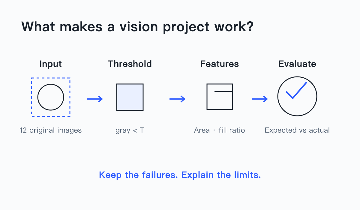
Cover the upper-right corner of a square, and this vision program calls it a circle. Its bounding box is exactly right, but its label is wrong: the remaining shape has a fill ratio of 0.759345, almost the same as the complete circle’s 0.755073.
That makes a useful first computer vision project. You can control the inputs, inspect intermediate values, and trace each failure to a specific decision. The task here is to recognize circles and squares in grayscale images, returning their count, labels, and bounding boxes. Twelve original synthetic images vary brightness, size, occlusion, and object contact.
The experiment is version 1.0.0, run with Python 3.9.6 and the standard library. It uses no trained model, weights, or image uploads. The numbers below come from actual runs. Synthetic images let us control conditions; camera photographs would need a separate evaluation.
Define a task you can score
“Build image recognition” leaves too much open. This project takes a 160 × 120 grayscale raster with values from 0 to 255. The background is lighter than the shapes. Complete shapes are axis-aligned and stay inside the image. The detector receives only the pixel array, without the generator’s saved labels or coordinates.
Each detected object carries inspectable data:
{
  "label": "circle",
  "bbox": [54, 34, 53, 53],
  "area": 2121,
  "fill": 0.755073,
  "aspect": 1.0
}
bbox means [x, y, width, height], measured from the upper-left corner. area counts foreground pixels in a connected component, fill divides that area by its bounding-box area, and aspect is the box’s width-to-height ratio. The detector can also return unknown or an empty list.
The generator stores ground truth separately, for evaluation. Occluded samples retain the identity and original bounding box of the complete object. The task is to recognize an occluded square, so identifying only its visible outline carries a corresponding error. Set this policy before interpreting results.
A scene passes when detection count matches ground truth, every object receives a one-to-one match, all matched labels are correct, and every matched box has intersection over union, or IoU, of at least 0.50. A blank scene passes only with no detections. This separates “correct location, wrong class” from “two objects merged into one box.”
Make original inputs with traceable answers
Download the complete reproduction package and extract it into its own directory.
| File | Purpose |
|---|---|
experiment.py | Generate samples, run two threshold methods, evaluate, and save results |
verify.py | Check saved PNG pixels, stable reruns, and the key misclassification |
viewer.html, viewer-template.html | Inspect saved inputs, boxes, and intermediate values in a browser |
results/inputs/*.png | All 12 original input images |
results/report.json, results/results.csv | Full numerical results and a comparison table |
checksums.json | SHA-256 hashes of generated artifacts |
With an existing Python 3 environment, run:
python3 experiment.py
python3 verify.py
python3 -m http.server 4342 --bind 127.0.0.1
Open http://127.0.0.1:4342/viewer.html. Select a sample and threshold method to inspect them. The viewer displays saved Python results and draws images and boxes with Canvas. Changing a menu does not train a model or rerun detection. After changing samples or rules, run experiment.py again and refresh the page. Stop the local server with Ctrl+C when finished.
Generation uses no randomness. Large circles have a radius of 26 pixels; large squares are 53 pixels wide. A circle includes pixels whose centers lie within the radius. Its bounding box is therefore 53 × 53, while its foreground area is 2121. The resulting fill ratio is about 0.755, rather than the continuous geometric value π/4.
The set contains a clean circle and square, a dim-background pair, a low-contrast pair, a small pair, an occluded pair, one scene with two touching circles, and one blank scene. The touching scene has two ground-truth objects and the blank has none, giving 12 objects across 12 scenes.
The detector’s input and the saved PNG originate from the same original pixel array. The verification script independently decompresses each saved PNG, reads its pixels, runs detection again, and compares the output. That connects the downloadable image bytes to the reported numbers.
Expose four stages of the data flow
The first stage is thresholding. The baseline marks pixels below gray level 180 as foreground:
threshold = 180
mask = [pixel < threshold for pixel in pixels]
The second stage finds four-connected components. Starting from a foreground pixel, a queue visits its left, right, upper, and lower neighbors until it has traversed the component. Diagonal contact behaves differently depending on the connectivity definition; this version uses four neighbors. The queue uses Python’s collections.deque.
The third stage extracts features and assigns labels. Components smaller than 64 pixels are discarded. Remaining objects must have an aspect ratio between 0.85 and 1.15. Within that range, a fill ratio from 0.70 to 0.88 produces circle, while a ratio of at least 0.90 produces square. Other cases produce unknown.
fill = area / (bbox_width * bbox_height)
aspect = bbox_width / bbox_height
label = "unknown"
if 0.85 <= aspect <= 1.15:
    if 0.70 <= fill <= 0.88:
        label = "circle"
    elif fill >= 0.90:
        label = "square"
These are deliberately simple baseline rules. They compress different outlines with similar occupied areas into the same feature values. Occlusion provides an immediate test of that choice.
The fourth stage evaluates the output. IoU divides the intersection of two boxes by their union. Candidate matches are sorted by decreasing IoU and assigned one to one; labels are checked afterward. This small experiment uses greedy matching. More crowded scenes may need a different assignment strategy.
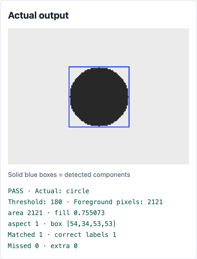
The clean circle passes count, location, and label checks, with the classification features visible alongside it.
Change brightness and inspect where the pipeline breaks
Normal samples use a background of 235 and a shape value of 40. Threshold 180 separates them. Dim samples use background 100 and shape 60. Both values fall below 180, so all 19,200 pixels become one component. Its box is [0, 0, 160, 120] and its class is unknown.
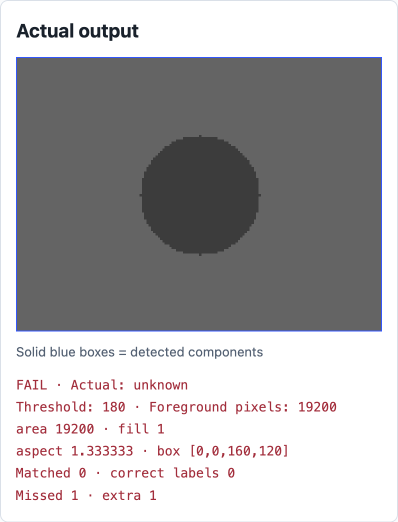
The background joins the foreground. This failure starts at segmentation.
For these uniform-background images, the upper-left pixel is guaranteed to be background. A direct change is to subtract 20 from that pixel’s value:
threshold = max(0, pixels[0] - 20)The dim samples now use threshold 80: background 100 is excluded and shape 60 remains. Normal and low-contrast samples use threshold 215, which also retains shapes with gray level 210. All later stages and classification parameters remain the same, so the comparison isolates the threshold change.
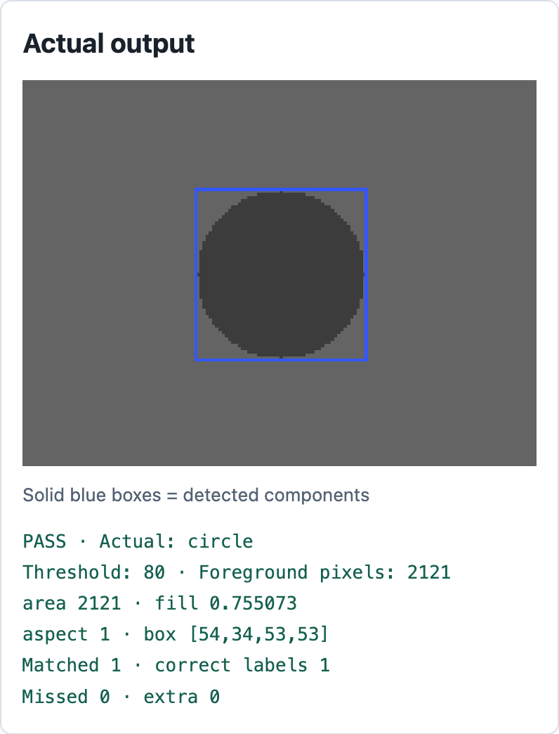
For the same input, changing only the threshold reduces foreground pixels from 19,200 to 2121.
This simulates whole-image brightness and contrast changes. The images contain no gradient shadows, reflections, or noise. The method may fail if an object covers the corner, the background varies spatially, or foreground and background differ by 20 or less. Local thresholds and multiple background samples are possible next experiments; they were not tested here.
Keep successes and remaining failures in the same table
Both methods use the same images and pass criteria:
| Input condition | Fixed threshold 180 | Background minus 20 |
|---|---|---|
| Clean circle / square | Both pass | Both pass |
| Dim circle / square | Whole-image unknown in both | Both pass |
| Low-contrast circle / square | No detections in either | Both pass |
| Small circle / square | No detections in either | No detections in either |
| Occluded circle | unknown, wrong label | Same failure |
| Occluded square | circle, wrong label | Same failure |
| Two touching circles | One unknown component | Same failure |
| Blank | Pass | Pass |
Fixed thresholding passes 3/12 scenes; background-relative thresholding passes 7/12 scenes. Of the 12 ground-truth objects, location matches meeting the IoU cutoff increase from 5 to 9, and correctly labeled objects increase from 2 to 6. Scene pass rate and correctly labeled object count use different denominators; the blank scene contributes to the first metric.
The comparison establishes that this change fixes four brightness-related failures in the controlled set. The same inspected samples were used for the adjustment, with no independent holdout set. Treat 7/12 as a regression result for these samples, rather than an estimate of accuracy on photographs.
The small circle has radius 4 and area 49. The small square is 7 pixels wide and also has area 49. Both are removed by the 64-pixel filter. Lowering the minimum area would let them reach classification, but the small circle occupies a 9 × 9 box and has fill 49/81 ≈ 0.605, outside the circle rule. Scale affects both filtering and the features produced by discrete pixels.
The occluded circle leaves a 33 × 53 box with aspect ratio about 0.623, failing the roughly square condition. Its IoU with the original box is also about 0.623, so its location matches while its label fails.
The most revealing misclassification is the occluded square. Removing a 26 × 26 patch from its upper-right corner leaves the 53 × 53 bounding box intact. Area falls from 2809 to 2133, moving its fill ratio into the circle interval. IoU is 1.0, yet the label is wrong.
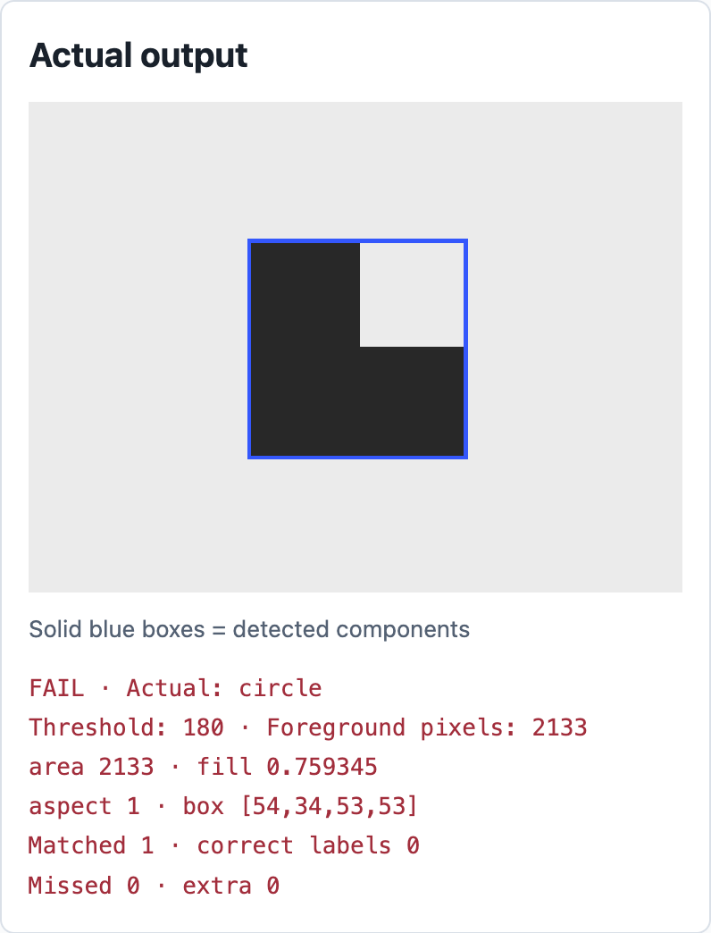
Fill ratio retains occupied area while discarding the concave corner and outline.
The touching circles share one edge pixel. Four-neighbor traversal merges them into a component with area 4241 and a 105 × 53 box. That merged box can match at most one answer. Its aspect ratio is about 1.981, giving unknown. A task that counts touching objects needs instance separation; further adjustment of the same global threshold does not address that failure.
Let failures choose the next investment
This project answers three practical questions: how the input becomes inspectable output, how success is defined, and where errors arise when conditions change. The next step depends on the intended task.
For consistently sized icons on clean backgrounds, the rules have explicit working conditions. Rotation, varied positions, and a little noise would make useful independent validation samples. Small icons need better treatment of scale in area filters and shape features. Occluded objects call for information about outlines, concavity, or templates. Natural photographs introduce a larger job involving acquisition, annotation, and an independent test set.
The package keeps every failure, along with input PNGs, full JSON, CSV, and source code. The actual verify.py run confirmed that all 12 saved images reproduce detections under both methods, reruns preserve artifact hashes, and the square-to-circle error remains in the report. Add a sample to SPECS, then trace it through thresholding, components, classification, and evaluation.
PNG output uses standard-library zlib compression. The viewer uses Canvas drawImage() to draw saved originals. Detection rules are implemented in the package’s own code. Every result has an input and a calculation you can revisit, giving the next change a concrete target to check.