OKLab, RGB, HSL and RYB: reproduce different palette paths
Compare encoded sRGB, shortest-hue HSL and OKLab with seven red-to-blue samples, inspect gamut clipping and reproduce a separate RYB approximation.
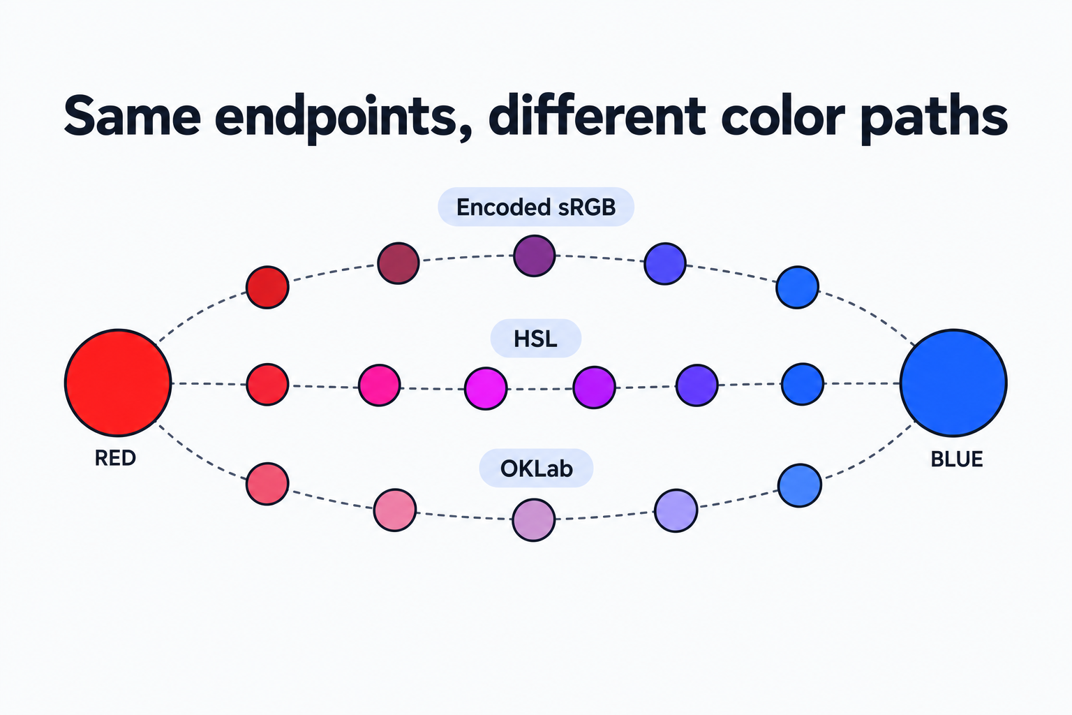
Put red #FF0000 and blue #0000FF at the ends of a gradient. What should sit in the middle? In this seven-color palette, encoded sRGB produces #800080, shortest-hue HSL produces #FF00FF, and OKLab produces #8C53A2. The endpoints agree; the coordinates and interpolation rules decide what happens between them.
Open the color-space palette preview to see the red-to-blue comparison immediately. Click either endpoint swatch to open a visual picker: drag in the color field, move the hue strip, or choose a common color. All three paths update as you explore. Apply color keeps your choice; Cancel or Esc restores the color from before you opened the picker. Each row contains seven samples, including both ends, at t = i / 6. Copy report copies the model names, version, endpoints and samples together.
A separate RYB example appears below. It uses preset RYB model coordinates independently of your selected endpoint colors. You can first obtain a reproducible digital palette, then decide which path suits your work.
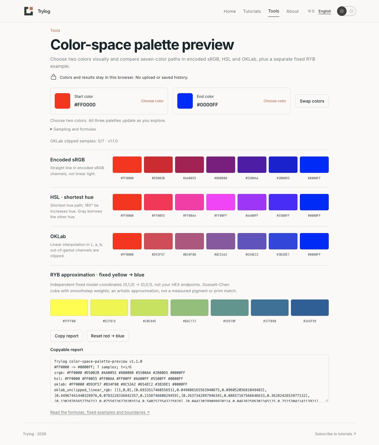
Three paths share the same HEX endpoints; the fixed RYB sample appears separately below.
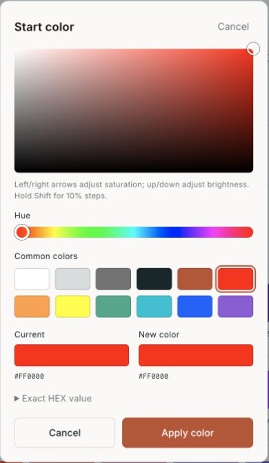
Choose visually and preview immediately, then apply. Exact HEX entry is available in the collapsed section.
Compare the same seven positions
To reproduce an exact color, expand Exact HEX value inside the picker. It accepts opaque six-digit sRGB HEX values, including letter case and surrounding whitespace. Named colors such as red, shorthand #F00, eight-digit colors with alpha, and Display-P3 values are outside the input range. Incomplete or invalid text leaves the last valid color visible; completing it updates the preview immediately. You can also cancel the selection. Arrow keys adjust saturation and brightness in the color field; hold Shift for larger steps.
The red-to-blue example produces:
| Position | Encoded sRGB | Shortest-hue HSL | OKLab |
|---|---|---|---|
| 0 | #FF0000 | #FF0000 | #FF0000 |
| 1/6 | #D5002B | #FF0055 | #D93F57 |
| 1/3 | #AA0055 | #FF00AA | #B34F80 |
| 1/2 | #800080 | #FF00FF | #8C53A2 |
| 2/3 | #5500AA | #AA00FF | #654EC2 |
| 5/6 | #2B00D5 | #5500FF | #3B3DE1 |
| 1 | #0000FF | #0000FF | #0000FF |
The reproduction package contains the core source, fixed inputs, full outputs and licenses. HEX channels are rounded to the nearest 8-bit integer. That final quantization changes an encoded channel by at most 0.5 / 255 after clipping. These values describe the algorithm; their appearance also depends on your display and viewing environment.
RGB: define which values form the straight line
Divide each HEX channel by 255. The encoded sRGB row then computes:
C(t) = (1 − t) × C0 + t × C1At t = 1/2, red and blue yield encoded channels (0.5, 0, 0.5). Multiplying by 255 and rounding produces (128, 0, 128), or #800080. This is a straight line through nonlinear sRGB-encoded values.
A linear-light average needs a decode–mix–encode sequence. CSS Color 4 specifies the sRGB conversions. The decoding function used here is:
c ≤ 0.04045: linear = c / 12.92
otherwise:  linear = ((c + 0.055) / 1.055) ^ 2.4
The average of linear red and blue is also (0.5, 0, 0.5), but those numbers now represent linear light. Encoding them gives approximately (0.735357, 0, 0.735357) and #BC00BC. That explains why two implementations described as “RGB mixing” can produce different purples. The tool labels its row “Encoded sRGB” and uses that convention consistently.
HSL: which way around the hue circle?
HSL is derived from encoded sRGB. Red has coordinates (0°, 1, 0.5) and blue (240°, 1, 0.5). The shortest route decreases hue by 120°. Its midpoint is 300°, producing saturated magenta #FF00FF. Increasing hue by 240° would instead take the longer route through green; this tool uses the short route.
The tool normalizes the hue difference to the shortest arc, then interpolates saturation and lightness linearly. At an exact 180° tie, it consistently chooses increasing hue. An achromatic endpoint borrows the other endpoint’s hue because its own hue has no visible meaning. When both endpoints are gray, hue is set to 0° and does not affect the result. For example, the HSL midpoint from #808080 to #FF0000 is #BF4040.
HSL’s L is the average of max(R,G,B) and min(R,G,B). It is useful for color controls, but equal L values across different hues do not ensure equal perceived brightness. The brighter-looking HSL midpoint in this example follows from both the model and the chosen hue path.
OKLab: interpolate in perceptual coordinates
Björn Ottosson’s original OKLab article supplies the conversion matrices and implementation license. This tool uses its updated coefficients in the following sequence:
- Decode sRGB into linear RGB.
- Transform linear RGB into three LMS components, then take their cube roots.
- Apply a second matrix to obtain OKLab
L, a, b. - Interpolate those coordinates independently, then invert the transformation to linear RGB.
- Clip out-of-gamut channels, encode sRGB, and round to 8-bit HEX.
Red is approximately (0.627955, 0.224863, 0.125846) and blue (0.452014, −0.032457, −0.311528). Their OKLab midpoint is approximately (0.539985, 0.096203, −0.092841). OKLab L has a different definition from HSL L; the two cannot be substituted for each other.
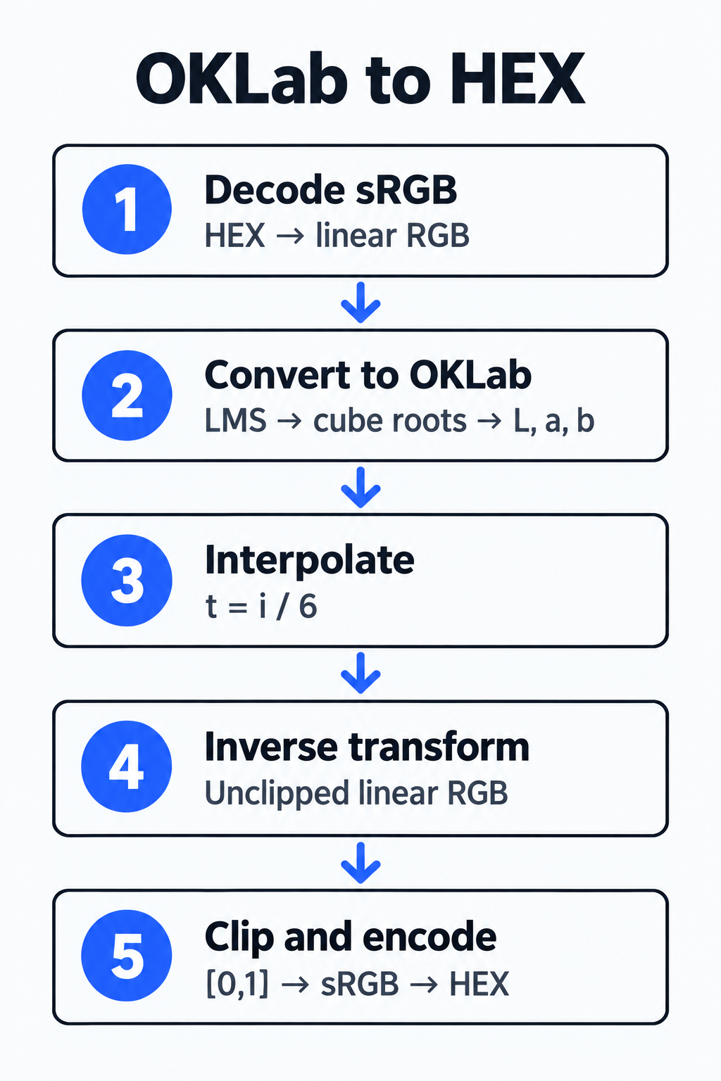
Calculate in OKLab, then map the result back to the supported sRGB output.
Along the unclipped OKLab line, consecutive samples have equal Euclidean coordinate distances. This offers a useful perceptual model for discussing a palette. The visible differences still depend on the colors, background, observation conditions and final quantization.
What happens outside the sRGB gamut?
Valid sRGB endpoints do not ensure that every OKLab intermediate lies inside sRGB. Change the inputs to #00FF00 and #0000FF to reproduce an out-of-gamut example. The tool retains each inverse-transformed linear RGB triple and marks a sample “clipped” when a channel leaves [0,1]. Matrix residuals smaller than 1e−7 do not count toward clipping; endpoints preserve their input bytes directly.
All five interior green-to-blue samples are clipped. The midpoint has linear RGB approximately (-0.081989, 0.400426, 0.519384); setting its red channel to 0 produces #00AABF.
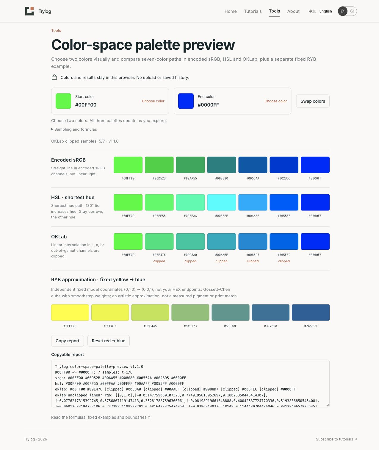
All five interior green-to-blue samples are marked clipped. The copied report retains their unclipped linear channels.
For display, negative channels become 0 and channels above 1 become 1, followed by encoding to HEX. Direct channel clipping is simple and deterministic. It can alter the equal-distance path and shift hue or chroma in the affected part. This tool does not implement perceptual gamut mapping. The reproduction package includes the raw linear channels so you can identify the affected samples.
RYB: a separate approximate color cube
The RYB example comes from Nathan Gossett and Baoquan Chen’s original manuscript, Paint Inspired Color Compositing. It aims to approximate red–yellow–blue mixing expectations from art education. Eight RYB cube corners are assigned RGB colors, then weighted to obtain intermediate values. Section 2.1 explicitly describes an approximation; Appendix A supplies the numerical corners and smoothing function:
u(t) = t² × (3 − 2t)
weight(corner) = product of u(axis) or (1 − u(axis))
RGB = sum of corner RGB × corner weight
The implementation here independently reproduces the Appendix A corner model. A numerical example in section 2.1 differs from the appendix: for (1, 0.5, 0.25), the appendix yields (0.8984375, 0.21828125, 0.0390625), while the text lists (0.886719, 0.212891, 0.039063). The package preserves the exact corner data and calculations used here so that this boundary can be checked.
The tool’s fixed path runs from RYB (0,1,0) to (0,0,1), producing:
#FFFF00 #ECF816 #C0E445 #8AC173 #59978F #377098 #2A5F99Yellow is #FFFF00; the appendix’s blue corner (0.163, 0.373, 0.6) becomes #2A5F99. The midpoint is the greenish #8AC173. Its blue endpoint differs from the #0000FF used in the digital comparison, so each example is explained using its own coordinates and endpoints. The tool does not invert arbitrary HEX values into RYB.
This RYB path is useful for exploring artistic palette ideas. Real pigments vary with composition, proportions, medium, substrate and illumination. Pigment recipes or print matching need relevant measurements and color-management information.
Keep the result in your own workflow
Try two brand colors, copy the report for the row you prefer, and test the palette against your actual background and text sizes. Text readability also needs a separate contrast check; a palette path does not supply an accessibility verdict.
The tool computes in the current browser without file uploads, result URLs or saved history. Its calculation button remains disabled if JavaScript fails to load. If clipboard permission is blocked, select the report and copy it manually. The report carries a model version, making gamma conventions, hue paths and clipping rules easier to compare with another implementation.
The topic was prompted by a Colorschemer author’s request for color-wheel feedback. The post raised questions about palette management, OKLab and RYB mixing. This article uses public formulas to build an independent tool and examples. Colorschemer’s desktop product was not tested. The download includes an MIT license for the original implementation and Ottosson’s license notice, with no third-party paper or product assets.