Database optimization with a reproducible SQLite index test
Compare query plans, ordered results and repeated warm-cache timings before and after a composite SQLite index on 200,000 synthetic orders.
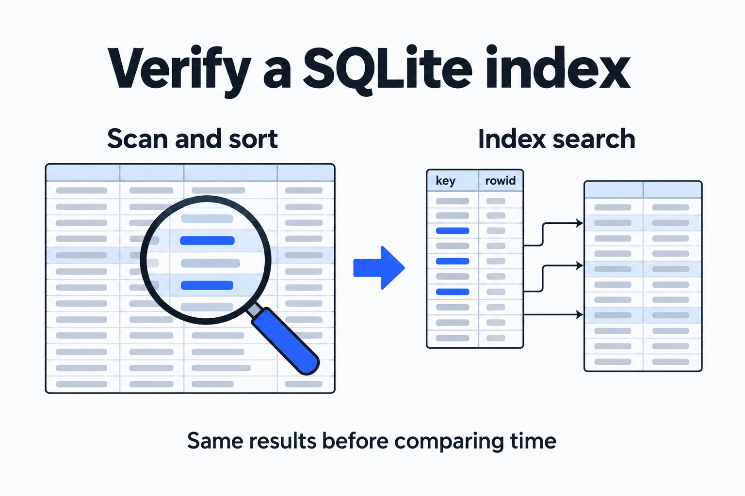
Database optimization can start with one query: preserve its data and parameters, inspect the plan, add an index for a specific reason, and compare results and repeated timings. This test uses 200,000 synthetic SQLite orders to retrieve a customer’s latest 20 paid orders within a time range. A composite index changed the plan from a full scan plus temporary sorting to an index search. In this warm-cache run, median time fell from 4.837 ms to 0.02254 ms, with every ordered result row unchanged.
Those numbers describe one local read-query fixture. The inputs, plans and measurement method below let you reproduce the test and examine why the index helps.
Fix the data and the question
The table contains 1,000 synthetic customers, three rotating statuses and timestamps increasing by 60 seconds per row. A note of 128 ASCII characters gives each row some width; the query does not read that field. Here are the schema and deterministic generation rule:
CREATE TABLE orders (
  id INTEGER PRIMARY KEY,
  customer_id INTEGER NOT NULL,
  status TEXT NOT NULL,
  created_at INTEGER NOT NULL,
  total_cents INTEGER NOT NULL,
  note TEXT NOT NULL
);
# i ranges from 0 to 199999
row = (
i + 1,
i % 1000,
['paid', 'pending', 'cancelled'][i % 3],
1700000000 + i * 60,
100 + (i * 7919) % 100000,
'x' * 128,
)There are 200,000 rows generated by a fixed formula. Amounts use integer cents. The created_at values are synthetic Unix seconds used only to define the range and ordering. The full script inserts these rows into a new temporary database, without connecting to an existing database.
The query and bound parameters are:
SELECT id, created_at, total_cents
FROM orders
WHERE customer_id = ? AND status = ? AND created_at >= ?
ORDER BY created_at DESC, id DESC
LIMIT 20;
params = (42, 'paid', 1703000000)Three conditions filter the rows, then the query returns the first 20 ordered by descending time and id. Using id as a second ordering key makes the order explicit even if timestamps tie. All timestamps in this dataset are distinct, but the additional key keeps the query’s meaning deterministic. These conditions match 50 rows and return 20 after LIMIT.
Read the plan before choosing the index columns
In Python, obtain the plan details with connection.execute('EXPLAIN QUERY PLAN ' + query, params). Before the index, the actual output was:
SCAN orders
USE TEMP B-TREE FOR ORDER BY
SCAN orders describes reading the full table in this plan. USE TEMP B-TREE FOR ORDER BY indicates a temporary B-tree for sorting. The SQLite EXPLAIN QUERY PLAN documentation defines these markers and warns that the output format may change across versions. The plan describes how rows are accessed; elapsed time still needs measurement.
This query fixes customer and status, restricts time, and takes the latest records ordered by time and id. The tested index follows that sequence:
CREATE INDEX idx_orders_customer_status_time
ON orders(customer_id, status, created_at DESC, id DESC);
The resulting plan was:
SEARCH orders USING INDEX idx_orders_customer_status_time
(customer_id=? AND status=? AND created_at>?)
The customer and status equalities narrow the search to the relevant index region, while time bounds it further. The final two columns follow ORDER BY, and the temporary-sort marker disappears. The multi-column search and sort section of SQLite’s query-planner documentation explains this mechanism.
The index excludes total_cents, so the plan says USING INDEX rather than a covering index. Fetching the amount still requires table access. This test begins with an index sufficient to change the access path; adding more columns needs a separate assessment of read and write load and storage.
Check equality before timing
The script copies one populated database, already processed by ANALYZE, into two versions. One remains unchanged; the other gets the index and another ANALYZE. Separate connections use identical parameters. Their first complete ordered result lists are compared directly, and every timed execution is also compared with the baseline list.
All 20 ids, timestamps and amounts matched, in the same order. The saved result’s SHA-256 is c79f414a4da97708ca6499630a96ab92bef4d7590ea698c2d95dc58671698570. The hash helps compare reruns; the correctness assertion uses full-list equality rather than row counts alone.
Each connection gets five warmups. Thirty executions before indexing and thirty after indexing are mixed and shuffled with seed 714. Timing surrounds only execute and fetchall:
start = time.perf_counter_ns()
rows = connection.execute(query, params).fetchall()
elapsed_ms = (time.perf_counter_ns() - start) / 1e6
assert rows == expected_rows
Data insertion, file copying, index creation, ANALYZE and the equality assertion are outside the query timer. Calling fetchall consumes every returned row, avoiding a measurement of query preparation alone.
Interpret this run
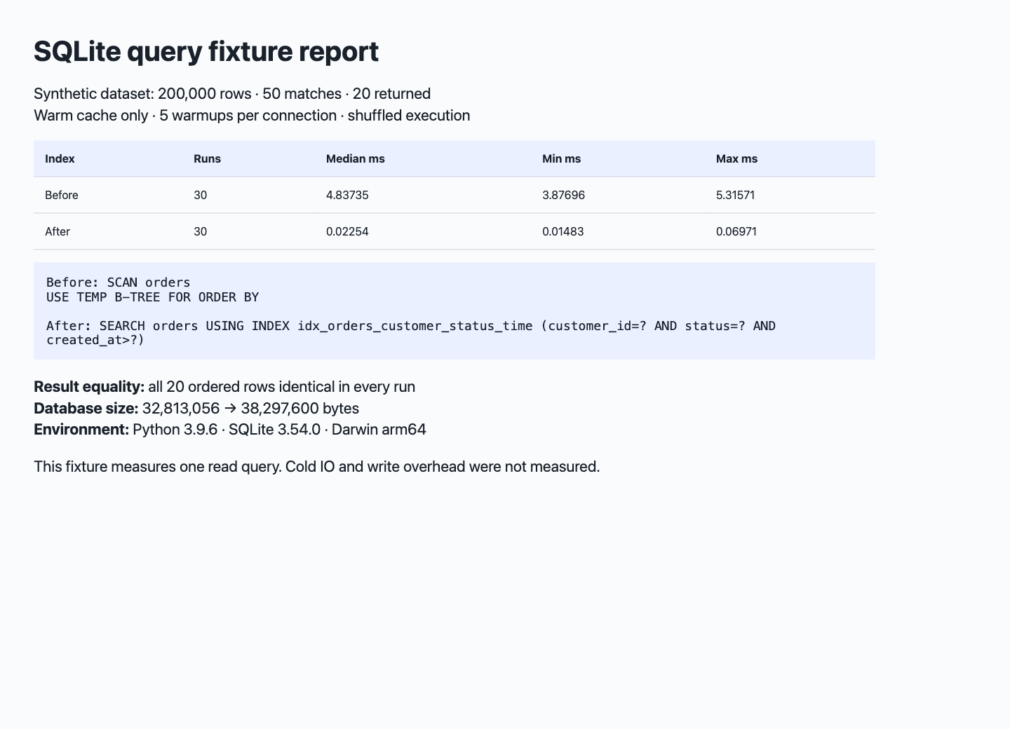
Local synthetic-data report showing the observed plans and warm-cache timings.
| State | Median ms | Minimum ms | Maximum ms |
|---|---|---|---|
| Without composite index | 4.83735 | 3.87696 | 5.31571 |
| With composite index | 0.02254 | 0.01483 | 0.06971 |
The environment was Darwin arm64, Python 3.9.6 and SQLite 3.54.0, with 4,096-byte SQLite pages. Each connection had a page-cache target of 65,536 KiB. Automatic indexes were disabled to keep the comparison focused on the explicit index. The operating-system cache was not cleared, so these are warmed-query measurements; cold disk reads remain unmeasured.
The lower indexed median is consistent with the plan’s reduced scanning and sorting. It describes this dataset, parameter set and result size. A different customer distribution, larger result set, changed ordering or a working set too large for cache can change the benefit.
Storage changed too: the database grew from 32,813,056 to 38,297,600 bytes, an increase of 5,484,544 bytes, approximately 5.23 MiB. Creating and committing the index took 59.38 ms in this run, excluding the subsequent ANALYZE. Ongoing inserts, updates and deletes must maintain the index. This fixture did not measure their cost or concurrent load; before adopting an index in a live application, measure critical writes and other common queries under a consistent method.
Run it on your machine
Download the complete script. It needs Python 3 and its built-in sqlite3 module:
unzip sqlite-index-fixture.zip -d sqlite-index-fixture
cd sqlite-index-fixture
python3 reproduce.py results
The script creates temporary databases and removes them after testing. Only JSON is retained in results, including complete plans, every timing sample, parameters, ordered rows, environment and file sizes. On a rerun, check equality and plan changes first, then compare times under the same machine conditions. Millisecond values need not match across machines.
The official CREATE INDEX syntax is another useful reference. Find more practical records in Workflows and methods.